How to make a vacation schedule in Excel Download Example
As the heat continues outside, the vacation season is in full swing. Today's article will be relevant as we show you how to check how many employees are working on a given day and whether it's sufficient. This is a question one of the website readers wanted to find an answer to.
Of course, the method presented here will be useful for those of you working in the HR department or, for example, in the sales or customer service department, as well as for entrepreneurs.
How to Create a Vacation Schedule Chart Template in Excel
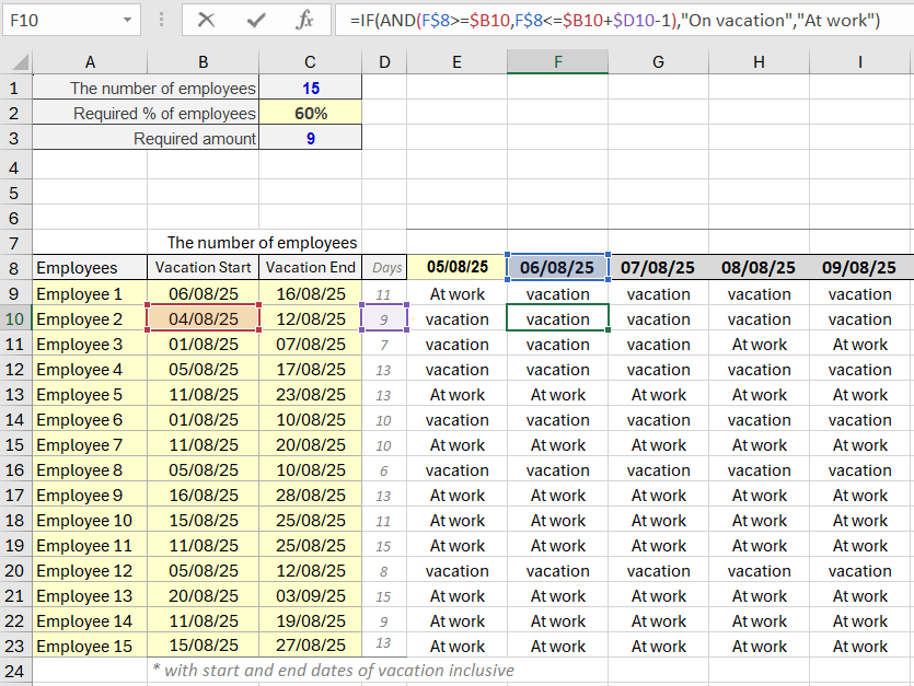
Let's assume that there are 15 people working in the sales department. We want at least 60% of the total to work daily, i.e., 9 people. If this condition is not met, the Excel vacation schedule template should notify about the shortage (it will indicate the shortage and highlight the cell borders in red).
The ready template looks like this (download at the end of the article):
Now, let's show you how to do it!
Initial view of the vacation schedule template at the initial development stage:
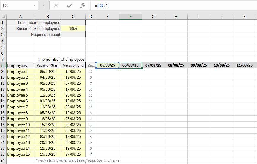
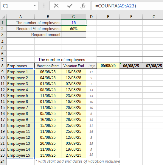
Firstly, let's calculate how many people are listed in our department on the graph. Enter the following formula in cell C1:
=COUNTA(A9:A23)
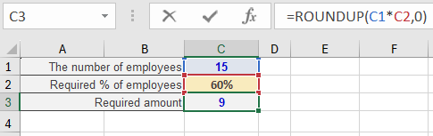
Now, let's calculate how many people make up 60% of the number of department employees (everyone except those on vacation). Enter the following formula in cell C3:
=ROUNDUP(C1*C2,0)
Great. The next step is to write a formula that will determine whether the employee is working on a given day or is on vacation. To quickly insert this formula automatically into the vacation schedule for all employees and all days, follow these steps:
- Select the range of cells E9:R23.
- Press the F2 key on the keyboard and enter the following formula:
- Confirm entering the formula by using the Ctrl + Enter key combination. As a result, all cells in the range E9:R23 on the schedule will be filled with the formula:
=IF(AND(E$8>=$B9,E$8<=$B9+$D9-1),"vacation","At work")
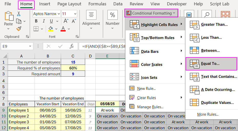
To make the vacation schedule template more readable and visually analyze it, let's add a conditional formatting rule:
- Select the range of cells E9:R23 again.
- Choose the tool: "HOME"-"Styles"-"Conditional Formatting"-"Highlight Cells Rules"-"Equal To".
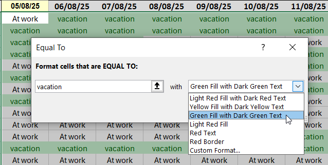
- In the appearing "Equal To" window, enter the value and choose the parameter as shown below:
- Click OK.
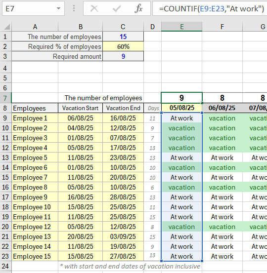
Next, we will calculate how many people are working on that day. To do this, fill the range of cells E7:R7 with the following formula:
=COUNTIF(E9:E23,"At work")
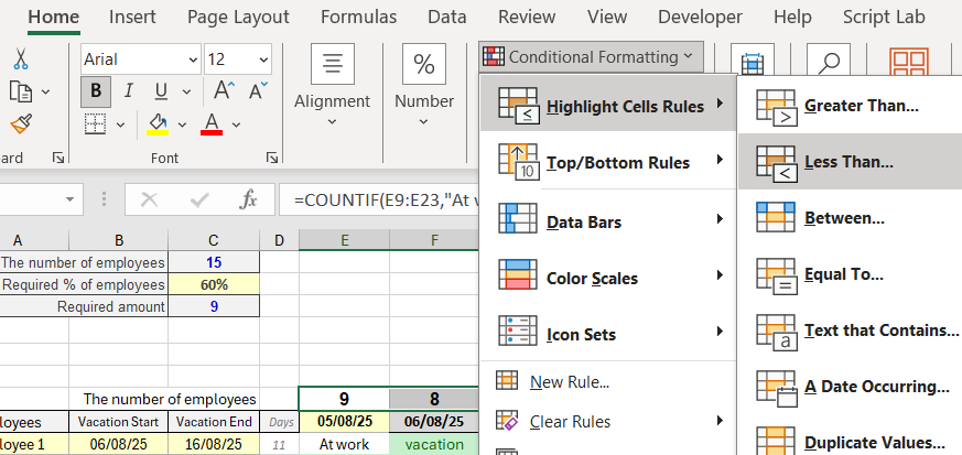
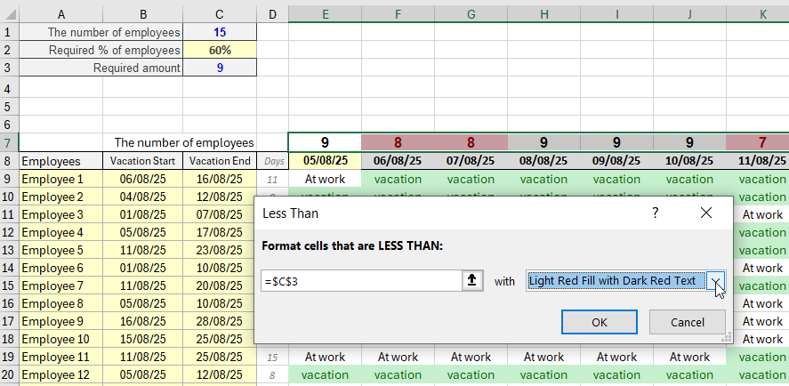
To this same range (E7:R7), assign our own conditional formatting rule. We need to add red borders every time there are too few employees on a particular day (less than 9 in our example). To do this:
- Select the range E7:R7 and choose the tool "HOME"-"Styles"-"Conditional Formatting"-"Highlight Cells Rules"-"Less Than".
- In the "Less Than" window that appears, enter the value and choose the parameter as shown below:
- Click OK to get the result.
Now let's determine what percentage of the whole team it is. Use the formula, which should be entered into the range of cells E6:R6:
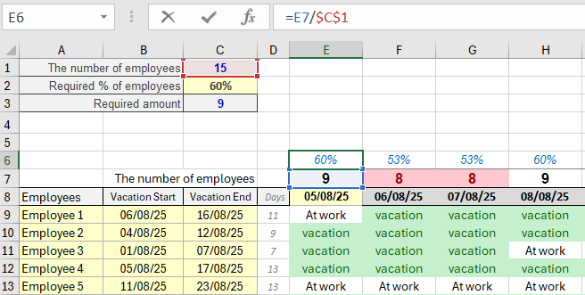
And finally: information on whether there is a shortage of employees or everything is fine? Use the formula for cells E5:R5:
=IF(E6<$C$2,"shortage","good")
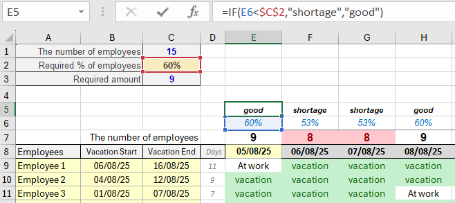
Finally, we have the following result:
We show only part of the data in the pictures. The attached file to this article has space for more days. Although we are confident that you will need even more.
 Download an example of how to create a vacation schedule chart in Excel
Do you know anyone who could use the information presented above? Send them an email with a link to this article. Most likely, they will find it helpful.

Data Visualization Charts for Interactive Report Creation in Excel.
Dashboard Templates