How SUMPRODUCT function works with a condition in Excel

The SUMPRODUCT function is one of the math and trigonometric functions that multiplies the corresponding elements of a given range of cells or arrays and returns the sum of the products.



Principles of working with multiple conditions in Excel

The syntax of the SUMPRODUCT function is as follows:

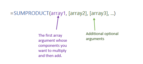
The first array is required. Values must be numeric, text values will be counted as 0 by the formula. Arrays 2,3 and so on are additional optional arguments and are used depending on the problem setting. This function multiplies several arrays by cells or by elements and sums the resulting products. The most common and simplest example of using the SUMPRODUCT function is to get the total cost by multiplying the price and the quantity of goods or services. In column B we have prices, and in column C we have quantities. We need to know the total cost of goods sold. In cell E4 we write the formula:

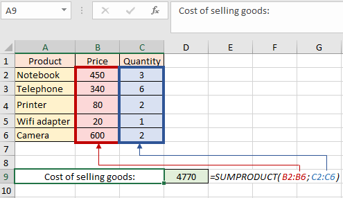
SUMPRODUCT multiplied the corresponding values from the two arrays (450*3; 340*6, and so on) in turn and summed the results. The SUMPRODUCT function supports working with arrays, which means that you can use the logic of array formulas using SUMPRODUCT. By the way, if you remember, to enter array formulas, you should always use the ctrl+Shift+Enter key combination. In our case, there is no need for this, since SUMPRODUCT works according to the logic of array formulas by definition. In the following example, we have a table that contains information about companies, their regions of operation, planned sales, and actual sales. Our task is to find out how many companies have completed the plan for the sale of goods or services. This problem can be solved in another way, for example, add a column in which to calculate the percentage of the plan, then apply COUNTIF or COUNTIFS. And this is a good and correct way, however, you can complete the task easier and faster. In cell E23 we write the formula:

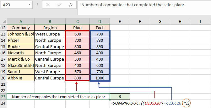
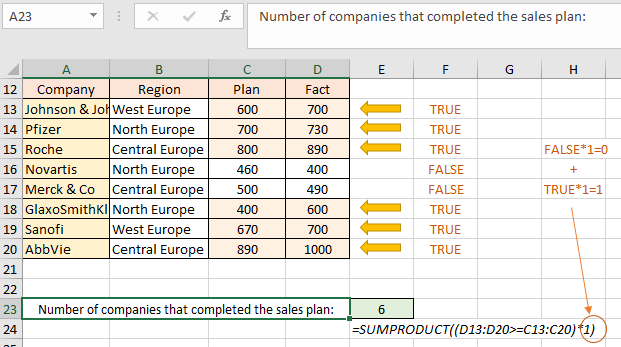
Thus, the condition D13:D20>=C13:C20 will be applied in turn to a pair of values in a row, then this comparison will return the Boolean false or true. In order to transform false and true into a numeric value, we multiply the condition contained inside SUMPRODUCT by 1. False*1=0, true*1=1. Then all received 1 are summed up:

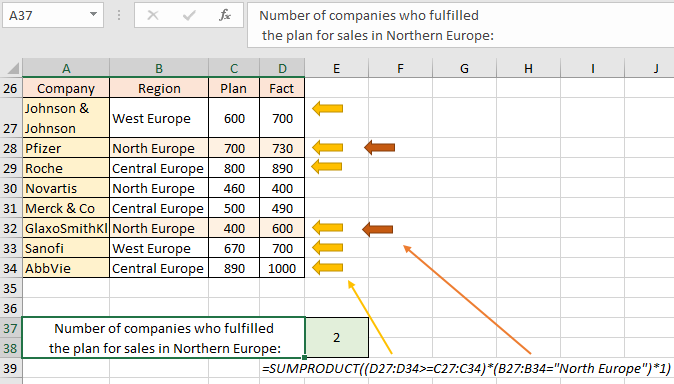
In the previous example, we used one condition, but you can add more conditions if necessary. For example, we need to find how many companies completed the plan in Northern Europe. To do this, we should add one more condition to the existing formula - the range B13: B20, the cells of which contain the text "Northern Europe":

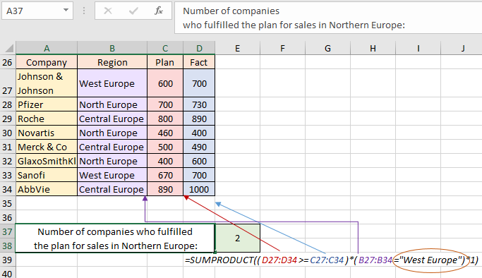
The text must be enclosed in quotation marks. The formula found companies that met the plan, then matched the found results with the second condition, left only those that matched and returned their number:



Summing subtotals in Excel by condition

Now let's say we need to count not the number of companies, but the total amount of actual sales of companies that meet the specified conditions of intermediate totals. To do this, we need to multiply the logical results not by 1, but by the corresponding sales volume. We replace the number 1 with a range that contains the following values:

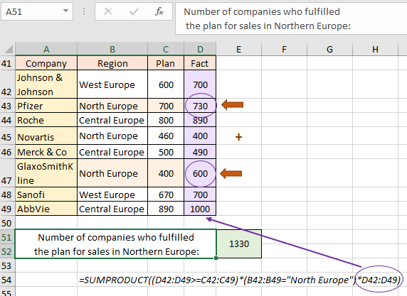
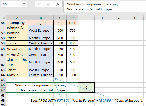
Now our TRUE will be multiplied by the corresponding sales value, and FALSE when multiplied will return zero. Functions that work with conditions are accompanied by logical operators AND, OR, NOT, and so on. If you look at our formula, the two given conditions are connected by a logical AND operator, that is, it searches for companies in which both the plan is completed and the location is Northern Europe. What if we need to link the conditions with a logical OR operator? Let's say we need to sum up the sum of companies from the regions of Northern and Central Europe. Then between the two conditions you need to put a plus sign instead of multiplication:

Selecting data from a range by several conditions in Excel

We have a table with data about employees and their scores received for testing skills. We need to choose among the employees those whose results turned out to be better than the rest. The first step is to calculate the average value. You can do it through the AVERAGE function and it will be correct:

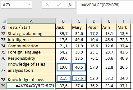
Now it seems like the leader has been determined, Jack, who has the highest average value. However, if we take a look at the overall score picture, we can see that Jack scored high in those categories that are not a priority for the performance of duties. And Maria, who is in second place, overtook Jack on the Knowledge of Sales Analysis Tools and Knowledge of Legislative Acts tests. That is, the weight of a certain test is important. We don't need an average, but a weighted average. In such cases, we use the SUMPRODUCT. We have another table that contains information about the weight of each test. In cell B80 we write the formula:

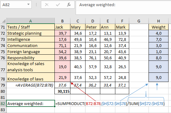
SUMPRODUCT multiplies and sums the score column and the weight column for each test. Then we divide the result by the sum of the values of column H. Do not forget to use absolute references for correct copying. Copy the formula to the end of the row:

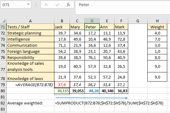
Now we are carefully looking at the results again - we have redefined the leader. In the previous example, Jack was in first place, now he has the lowest result. Maria went from second place to 3, and Peter turned out to be the leader.

How the SUMPRODUCT function works with text values in Excel

Another simple but working example of using:

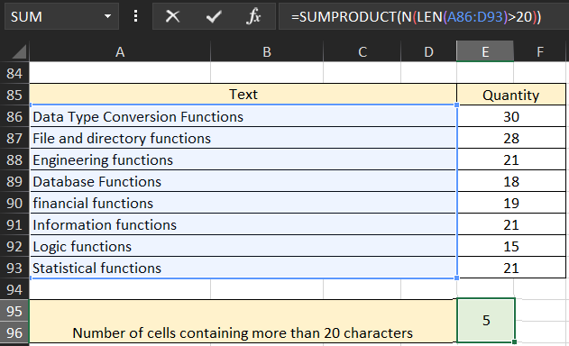
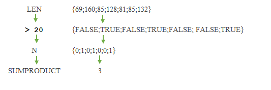
In this example, we have counted the number of cells whose content exceeds 20 characters. This formula works from the inside: LEN counts how many characters the text contains in a cell (the return result of the LEN function can be seen in column E). The elements from the array are then matched against the "greater than 20" condition and set to FALSE or TRUE. After that, the N function transforms the received logical results into the numbers 1 and 0. At the end, SUMPRODUCT counts the number of corresponding cells:

Download SUMPRODUCT examples with multiple conditions in Excel

In skillful hands, the principles of operation of the algorithms of the SUMPRODUCT function allow you to replace many other formulas and functions in Excel to automate the solution of the same tasks. Moreover, this function can work with data ranges in unopened Excel files (workbooks). Of the shortcomings, it is worth noting the inability to use wildcard characters * in criteria when processing text values. But this minus can be circumvented by combining the formula with text functions, which will work great at intermediate stages of processing criteria with conditions during the calculation.