Formula INDEX and MATCH with Multiple Search Criteria in Excel
A two-dimensional table is a rectangular range of cells, that is, a continuous range consisting of several rows and columns. To select values from two-dimensional tables, it is easy and convenient to use an effective formula that combines the INDEX and MATCH functions. The main disadvantage of this formula is the fact that it can only be applied to two-dimensional rectangular tables in a continuous range of cells. But in its field, this formula takes to water and creates great search tools for several user conditions.
Selecting Values Using INDEX and MATCH with Multiple Criteria
Below is a table depicting sales data by regions for four years. Each row represents a different regional area, and each column represents a different year. Suppose the user needs to extract values from the table based on two criteria:
- Select a region.
- Specify a year.
As a result, they should obtain the value from the corresponding row and column in the table, similar to a table like the Pythagorean Table:
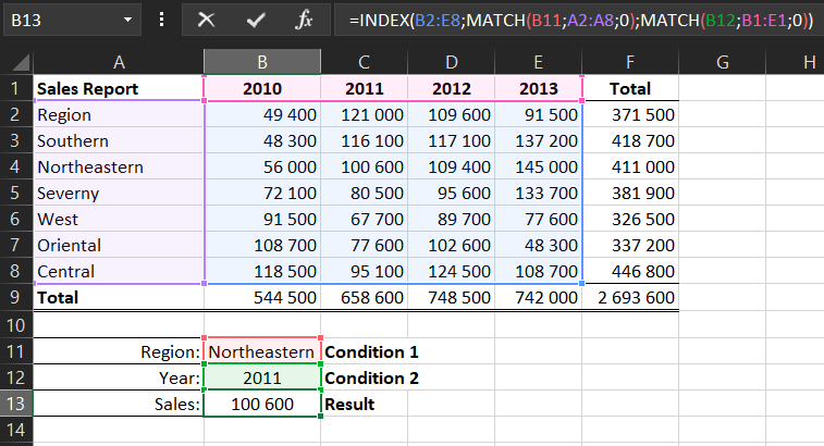
Most Excel users are familiar with the formula using the INDEX and MATCH functions. Unlike other formulas, here, two MATCH functions are used in the second and third arguments of the INDEX function because the search is based on two criteria. In the third argument, the "Column number" of the INDEX function, there is no constant value; instead, the MATCH function is used, which dynamically changes the value.
The MATCH function returns the position of the found value in the list. In the current selection of the "Northern" region, the function returns the value 3 because this region is in the third position in the list. This number is currently the value of the second argument of the INDEX function. The year 2011 is found in the table's header row. Since it's in the second position in the list, the MATCH function returns the number 2 for the third argument. Based on the numbers 3 and 2 returned by the MATCH function, the INDEX function returns the value that meets the user's specified criteria.
The Simplest Way to Select Values Based on Multiple Criteria in Excel
But what if all the multiple criteria need to be searched only vertically within the columns of the table?
The simplest way to use multiple criteria for the INDEX function is to concatenate ranges using the CONCATENATE function or simply the "&" symbol in the parameters of the MATCH function. This applies to both the first and second arguments of the MATCH function:
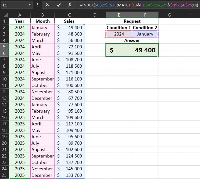
This same method works for horizontal value searches as well. In the second argument of the MATCH function, you specify the ranges for rows instead of columns.
Alternative Formula for INDEX and MATCH with Multiple Criteria
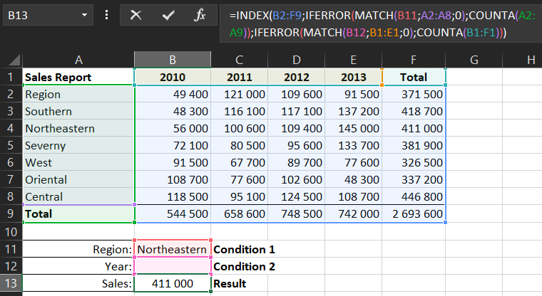
You can significantly expand the capabilities of the formula mentioned above. You can extract sales data from the table based on multiple criteria. This allows users to specify one of four criteria:
- Specify region and year (as in the previous example).
- Specify only the region.
- Specify only the year.
- Specify no criteria at all.
Now a new INDEX and MATCH formula with multiple criteria will be executed. The modified formula should still provide the correct final results without limiting the user.
For example, if none of the criteria for selecting sales data is specified, then the formula assumes that the user needs the total sales amount for all years and all regions as the final result. In other words, if the user does not specify custom criteria, the formula returns the total sum of all numbers in the table:
 Download INDEX and MATCH with Multiple Search Criteria in Excel
The overall structure of the modified formula is the same as in the previous example. Only a few details have changed. The range defined by the INDEX function now covers both row 9 and column F. Both MATCH functions have been modified and are additionally located in the IFERROR function's arguments. This function allows the formula to return the total sum of numbers either by rows or by columns, thanks to the inclusion of the total values in row B9:F9 and column F3:F9.
In the image, the same table is shown, but the user did not specify the "Year" criterion in cell B12. Since the row and column headers do not contain empty cells, the old formula returns an error with the #N/A code. At the same time, in the new modified formula, the situation is controlled by the IFERROR function, which returns a value from its second argument, "Value if Error." In this way, the INDEX function simply receives the number of the last column. If no region is specified, but the year is specified, the INDEX function takes the number of the last row in the original table and displays the content of cell F7 with the total sum.

Data Visualization Charts for Interactive Report Creation in Excel.
Dashboard Templates