How to Create 3 Linked Dynamic Dropdown Lists in Excel
So, how to create two linked dropdown lists in Excel: category, subcategory, and a lower-level category. In this case, in our own words, the lower level is the "sub-subcategory" if it exists at all. But for a better understanding of this tutorial, let's assume it exists.
Two Linked Dropdown Lists with an Array Formula
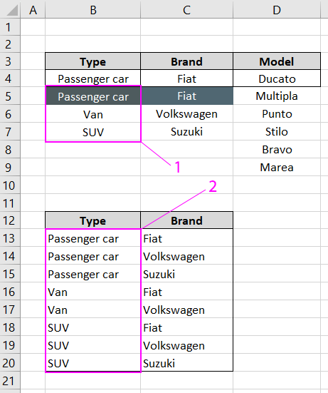
Anyway, let's start by mentioning that this tutorial is a continuation of the material: How to Create Dependent Dropdown Lists in Excel, where we detailed the logic and method of creating one of these lists. We recommend checking it out because here we will only describe how to create the other linked dropdown list :-) And this is what we want to achieve:
So, we have:
- Car type: Sedan, Van, and SUV (Category)
- Manufacturer: Fiat, Volkswagen, and Suzuki (Subcategory)
- Model: ... there are a few of them :-) (Sub-subcategory)
At the same time, we have the following data:
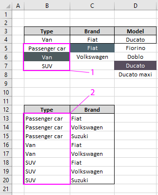
This list should be sorted in the following order:
- Type.
- Manufacturer.
- Model.
It can be of any length. What's also important: we need to add two smaller lists to it, necessary for Type and Manufacturer, i.e., for the category (first list) and subcategory (second list). These additional lists look like this:
The thing is, these lists should not have duplicate entries for Type and Manufacturer that are in the Models list. You can create them using the "Remove Duplicates" tool (for example, as shown in this approximately 2-minute video). When we've done that, then...
First and Second Linked Dropdown List: Type and Manufacturer
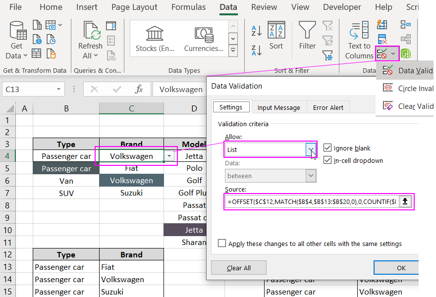
For the cells that should become dropdown lists, go to the "Data" tab, choose "Data Validation," and as the data type, select "List."
For Type, as the data source, we simply specify the range B7:B9.
For Manufacturer, we already use a formula, which is detailed here. It looks like this:
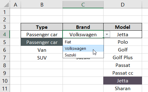
=OFFSET($C$12,MATCH($B$4,$B$13:$B$20,0),0,COUNTIF($B$13:$B$20,$B$4),1)
Model - we'll describe it in the same way.
Third Linked Dropdown List: Model
Now, let's see how to link a dropdown list in Excel. Since Model depends on both Type and Manufacturer, we will use a complex formula. After that, we'll place it not in data validation but in a named range. Accordingly, data validation will contain a reference to this name. Let's assume we want to display sedan models of Fiat. In the first list, we selected Sedan, in the second - Fiat.
We will move cell H4 down by as many rows as it takes to find the position of the first sedan Fiat. So in the Type column, we should have Sedan, and in the Manufacturer column, Fiat should be present. If we used an intermediate column (which would be an excellent solution, but we want to show you something cooler ;-), we would look for the combination of this data: Sedan Fiat. However, we don't have such a column, but we can create it "on the fly," in other words, using a formula. Typing this formula, you can imagine that such an intermediate column exists, and you'll see that it will be easier ;-)
To determine the position of Sedan Fiat, we will, of course, use the FIND function. See:
FIND(B4&C4;F5:F39&G5:G39;0)
This means that we want to know the position of Sedan Fiat (hence the link B4&C4). Where? In our imaginary auxiliary column, i.e., F5:F39&G5:G39. And here is the most challenging part of the whole formula.
The rest is simpler, and the COUNTIFS function deserves the most attention, which checks how many Sedan Fiats there are. In particular, it checks how many times in the list there are entries that in column F5:F39 have the value Sedan, and in column G5:G39 - Fiat. The function looks like this:
COUNTIFS(F5:F39;B4;G5:G39;C4)
And the entire formula for the named range of the dropdown list is:
=OFFSET($H$4,MATCH($B$4&$C$4,$F$5:$F$39&$G$5:$G$39,0),0,COUNTIFS($F$5:$F$39,$B$4,$G$5:$G$39,$C$4),1)
If you plan to use this formula in multiple cells, don't forget to mark the cells as absolute references!
Now, to use this formula correctly in the third dropdown list, we need to follow a series of steps:
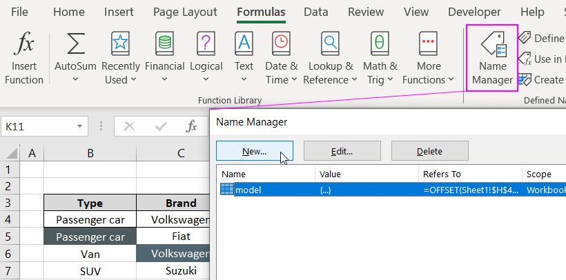
- Create a new name. To do this, select the tool: "Formulas" - "Defined Names" - "Name Manager" - "Create."
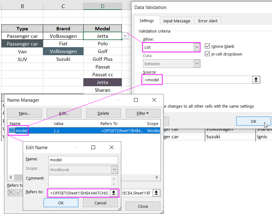
- When creating the name, in the "Name:" field, enter the word "model," and in the "Refers to:" field, enter the above formula and click OK in all open dialog boxes:
- Go to cell D4 to create a dropdown list, where this time in the "Source" input field, you should enter a link to the above-created name with the formula =model.
 Download
When you go to the "Data" menu, "Data Validation," and choose "List" as the data type, in the "Source" field, paste not the formula itself but a reference to the name "=model" of the named range with this formula. This approach ensures the stability of the third dropdown list.

Data Visualization Charts for Interactive Report Creation in Excel.
Dashboard Templates